black-hole.js
Black holes are one of the grand edge cases of nature, places where our understanding of quantum and classical mechanics breaks down. They have forced physicists to face some truly bizarre ideas, such as the possibility that our universe may be a hologram with all of its information stored on a massive two dimensional surface surrounding us. They are places of paradox: it might actually be true that explorers who venture across a black hole’s horizon may fly through without noticing a thing, while observers on the outside would observe the explorer getting thermalized and spread across the black hole’s horizon, and both histories may be right. Bizarre. Also, they look really cool.
In Nolan’s Interstellar, a giant black hole looms menacingly and majestically in space, its swirling light shows defying comprehension. The movie was my first introduction to the beauty of gravitational lensing, a concept I’d often read described in physics coursebooks but never seen demonstrated so compellingly. I decided recently that I wanted to learn how gravitational lensing worked and see if I could put such knowledge to use.
Thus in the time-honored tradition of taking yet another noun and making .js file out of it, I proudly present black-hole.js (see on GitHub), which uses a numerical ordinary differential equation solver from numeric.js, and some nice WebGL utilities from glfx.js, to render the gravitational lensing of a black hole.
Demo
Move your mouse around in the image below, and watch the black hole follow you.
What is gravitational lensing?
One of Einstein’s foremost contributions to physics was the idea that gravity not only attracts discrete masses to one another, it actually warps the fabric of space itself. This means that even infinitesimally lightweight photons are attracted to the heavy celestial bodies in the universe. Black holes are well known for the fact that their powerful gravity traps light itself within its horizon, making a spherical region of space completely devoid of light (hence their name). But you can imagine that rays of light that pass near the edge of the black hole might be bent in fiercely but perhaps not hard enough to be trapped.
There are several strange phenomena near the edge of the black hole. Elements far to one side of the black hole may show up near it on the other side due to the fierce warping of space. Light rays that bend very near the black hole’s horizon may actually wrap back around to the viewer, meaning that you should actually be able to see yourself in some of the light that bends around the black hole.
If we want to compute these gravitational lensing effects, we’ll need to dig a bit into the math of what is going on. There are some decent explanations and formulas for explaining gravitational lensing on Wikipedia, but the best summary I found was an excellent post by Jason at jasmcole.com. Feel free to visit his post to learn more about the physics of gravitational lensing in detail.
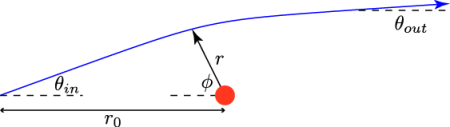
Space bends around a massive object. Source: jasmcole.com
If we have a light ray leaving the viewer toward the black hole at an angle \( \theta_{in} \), and the viewer is at a distance \(r_0\) from the black hole, it would be useful to determine the final angle \(\theta_{out}\) as the light recedes far away from the black hole. We can trace the ray’s path around the black hole in polar coordinates where \(r\) is the distance from the black hole and \(\phi\) is the angle between the photon and the axis between the viewer and the black hole. To my knowledge, there is not a closed-form solution relating \(\theta_{in}\) and \(\theta_{out}\), but, thanks to the physics expertise from Jason of jasmcole.com, here is a simple ordinary differential equation relating these quantities.
$$ \frac{d^2(1/r)}{d \phi^2} + \frac{1}{r} = \frac{3 G M}{c^2 r^2} $$
To simplify even further, we can substitute \(u\) for \(\frac{1}{r}\), and choose units such that \(G = M = c = 1\), giving us a very simple 2nd order ODE:
$$ \frac{d^2 u}{d \phi^2} = 3 u^2 - u $$
If we solve this ODE for a single value of \(\theta_{in}\), we can view the x-y coordinate photon path and analyze where the photon ends up. Repeating this for many values of \(\theta_{in}\) will provide enough data to create a mapping between \(\theta_{in}\) and \(\theta_{out}\). You can use MATLAB or similar tools to solve the ODE, but because I wanted to create a JavaScript widget and ultimately allow its parameters to be configurable, I resorted to using numeric.js, a cool mathematics library with a nice workshop REPL online that you can use to plot graphs and debug.
Solving a 2nd order ODE with numeric.js
The numeric.js library comes packed with many useful mathematical tools, which you can read about here, and try out in the online workshop REPL here. The one that is interesting for our use case is the numeric.dopri() function, which performs numerical integration of an ODE using the Dormand-Prince RK method. In other words, this function will take in an ODE and output a large series of points that fit the ODE constraints, which you can then plot.
Let’s see if we can get our ODE into a form that numeric.dopri() can accept. It expects our ODE to come in the form of a function with two parameters: the independent variable (in our case \(\phi\)), and a vector of two dependent variables, \(u\) and \( u^{‘} \), in our case. It then expects us to return a vector containing the values \( u^{‘}\) and \(u^{“}\). We can write down this ODE function as follows:
var blackHoleODESystem = function (phi, vec) {
  var u = vec[0];
  var u_prime = vec[1];
  var u_double_prime = 3*u*u - u;
  return [u_prime, u_double_prime];
}
In order to solve our ODE, numeric will need to know initial values for \(u\) and \(u^{‘}\). Simply enough, \(u_0 = 1/r_0\), and we can use some geometry to find that \(u^{‘}_0 = 1 / (r_0 \cdot tan (\theta_{in}))\). In my own experiments, I found that setting \(r_0\) to 20 yielded nice results. You can play with varying angles for \(\theta_{in}\) and see what the paths look like, but I found that \(\theta_{in} \leq 15^{\circ}\) yielded paths that fell into the black hole, and around \(16^\circ\) to \(18^\circ\) yielded paths that wrapped around and came back toward the viewer.
With our system and initial values determined, we can call numeric.dopri() to give us coordinates that match the ODE constraints:
var getBlackHoleSolution = function (startAngle, startRadius, startPhi, endPhi, optionalNumIterations) {
  var numIterations = optionalNumIterations || 100;
  return numeric.dopri(
    startPhi,
    endPhi,
    [1.0 / startRadius,
     1.0 / (startRadius * Math.tan(startAngle))],
    blackHoleSystem,
    undefined, // tolerance not needed
    numIterations
  );
}

var startAngleInDegrees = 15;
var startRadius = 20;

var sol = getBlackHoleSolution(
  startAngleInDegrees * Math.PI / 180,
  startRadius,
  0,
  10 * Math.PI
);
It’d be really nice to plot the x-y coordinates of this solution and watch the photon’s path around the black hole. Here’s a function that will do it.
var getXYPhotonPathFromSolution = function (sol) {
  // Note: transpose(sol.y)[0] contains the u values.
  // transpose(sol.y)[1] contains u_prime values.
  var rValues = numeric.transpose(sol.y)[0]
    .map(function (u) {
      // we want the radius r = 1/u
      return 1 / u;
    });
  var phiValues = sol.x;
  var photonPath = [];
  for (var i = 0; i < rValues.length; i++) {
    // Negative r is nonsensical, and this can occur as
    // radius goes to infinity. Stop when you start
    // hitting infinity
    if (rValues[i] < 0) break;
    var x = rValues[i] * Math.cos(phiValues[i]);
    var y = rValues[i] * Math.sin(phiValues[i]);
    photonPath.push([x, y]);
  }
  return photonPath;
}
Finally, we can plot this x-y photon path using numeric.js’s workshop REPL. You’ll need to copy the functions above into the REPL to make them available for your use there.
We can do a few operations in the REPL to plot our solutions. First, it is much easier to see your results if you set the bounds on the plot to be fixed, so first we set some default plot boundary options. Then, we create two solutions, one for a 15 degree light ray angle, and the other for a 40 degree angle. After that, we generate x-y photon paths for the two solutions. And finally, we plot the results.
> var plotOptions = { xaxis: { min: -20, max: 20 }, yaxis: { min: -20, max: 20 } }
> var sol1 = getBlackHoleSolution(15 * Math.PI / 180, startRadius, 0, 10 * Math.PI);
> var sol2 = getBlackHoleSolution(40 * Math.PI / 180, startRadius, 0, 10 * Math.PI);
> var photonPath1 = getXYPhotonPathFromSolution(sol1);
> var photonPath2 = getXYPhotonPathFromSolution(sol2);
> workshop.plot([photonPath1, photonPath2]);
Here is a plot of several angles. Paths that begin with small initial angles swirl around and fall into the black hole. Angles slightly larger than those would allow the viewer to see around corners. Finally, the largest angles are only moderately deflected.
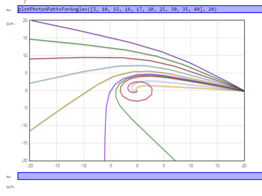
Rays of light spiral around a black hole. Screenshot from Numeric.js workshop REPL.
Creating a \(\theta_{in}\) to \(\theta_{out}\) fitted polynomial function
Now that we can produce the x-y photon path for a given \(\theta_{in}\), how can we use this path to find \(\theta_{out}\)? I found that assuming that sampling 100 initial angles between \(0^\circ\) and \(80^\circ\) works quite well. Given an x-y path for a photon, we do the following:
For small initial angles, there actually is no \(\theta_{out}\) because those photons actually fall into the black hole. To determine if an x-y photon path falls into a black hole, we check to see if its final coordinate is within a small distance of the black hole at \((0, 0)\). We will ultimately find the largest initial angle that fell into a black hole and record it. Ultimately, pixels with smaller corresponding initial angles will be drawn black in the final image.
For all other initial angles, the photon should end somewhere far from the black hole. We determine the final angle, \(\theta_{out}\) by simply taking the arc-tangent of the slope between the final two points on the x-y path. Some of the resulting angles will indicate that the ray is shooting outside the bounds of the image, or even looping back around toward the viewer. What you decide to ultimately paint into such pixels is up to you because, unlike in nature, we don’t have full 3D image information of the surroundings. I ended up simply clamping to the nearest boundary pixel, which looks fairly good.
Once we have the in-angle to out-angle lookup table, we can generate a fitted polynomial function with the assistance of the
numeric.uncmin()function. We can set up a “least squares” problem for numeric.js to optimize where the solution will choose coefficients for a polynomial function that will closely fit our data. I found that a simple 2nd degree polynomial function fit best. Here is the polynomial function:
$$ f(\theta_{in}) = c_0 + c_1 \theta_{in} + c_2 \theta_{in}^2 $$
Here is the algorithm that numeric.js will use to minimize the square of the difference between the function’s results and our data. It will iteratively choose good coefficients \( c_i \) until the function gets acceptably close to the data:
- Choose \(c_0\), \(c_1\), \(c_2\), defining a new polynomial function \(f\).
- Compute the following sum: \( \sum_{i = 0}^{n} (f(\theta_{in_i}) - \theta_{out_i})^2 \)
- Iteratively improve \(c_0\), \(c_1\), and \(c_2\) until the sum above is acceptably minimized.
Here’s what this process looks like in JavaScript:
var angleTables = computeBlackHoleTables(
  startRadius,
  numAngleDataPoints,
  maxAngle,
  optionalNumIterationsInODESolver
);

var polynomial = function (params, x) {
  var sum = 0.0;
  for (var i = 0; i <= polynomialDegree; i++) {
    sum += params[i] * Math.pow(x, i);
  }
  return sum;
}

var initialCoeffs = [];
for (var i = 0; i <= polynomialDegree; i++) {
  initialCoeffs.push(1.0);
}

var leastSquaresObjective = function (params) {
  var total = 0.0;
  for (var i = 0; i < angleTables.inAngles.length; i++) {
    var result = polynomial(params, angleTables.inAngles[i]);
    var delta = result - angleTables.outAngles[i];
    total += (delta * delta);
  }
  return total;
}

var minimizer = numeric.uncmin(leastSquaresObjective, initialCoeffs);

var polynomialCoefficients = minimizer.solution;
Using some geometry to render the result
The drawing below demonstrates the approach. It shows a possibility where, when trying to determine what should be painted to the location at the red dot in the final image, we find that we should paint the contents from the location of the green dot in the original image.
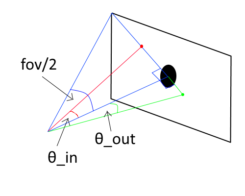
Since the light ray bends around the black hole, take the pixel at the output angle and paint it into the pixel at the input angle.
The algorithm works as follows. First, we need to determine the distance from the viewer to the image plane in “pixel space.” Since we’ve specified an FOV angle, that distance is \(B = diagonal/(2 \cdot tan(fov/2))\). Then, we can then compute the angle \(\theta_{in}\) for any x-y pixel coordinate.
$$
d = \sqrt{(x-x_{bh})^2 + (y-y_{bh})^2)}
\theta_{in} = arctan \frac{d}{B}
$$
Now that we have \(\theta_{in}\) for a given x-y pixel, how do we determine its corresponding \(\theta_{out}\)? We created a fitting polynomial function above, call it \( f(\theta_{in}) \). Simply call this function to get \( \theta_{out} \). If this \(\theta_{out}\) is less than the black hole angle, we paint black. If it is greater, we find its distance from the black hole center, \(d_{out} = B \cdot tan \theta_{out}\). This value may be negative or positive depending on the angle \(\theta_{out}\). If negative, then \((x_{out}, y_{out})\) will be on the opposite side of the black hole of \((x_{in}, y_{in})\). The x-y out-location can be found by creating a unit vector between the x-y in-location and the black hole, and multiplying it by the distance value \(d_{out}\).
And there you have it.
HTML5, WebGL, and shaders, oh my!
My first attempt to render the black hole in the browser was both exhilarating and disappointing. Using HTML5 Canvas and ImageData objects, I was able to produce a rendering of a static black hole in the center of a background image quite quickly. However, when I modified the plugin such that the black hole followed my mouse around the background image, the program stuttered badly, with approximately 300 - 400 ms of latency between each frame. I tried several HTML5 hacks, to no avail.
This rendering process seems inherently parallelizable, however. Initial angles mapped independently to output angles with no dependencies on computation from other neighbors. This should certainly be something that a GPU should be able to handle well. I decided that now was as good a time as any to learn a bit about WebGL GLSL shaders.
There was substantially more necessary boilerplate code involved in drawing things with WebGL than I’m used to as a web and mobile -focused engineer. I wanted to keep my WebGL code as succinct as possible, leveraging any other open source work I could so that my program could focus on the interesting gravitational lensing concepts. I found a very nice foundation to build on. The glfx.js library is fantastic. Their home page demo even prominently displays a swirling black hole-esque effect than follows the mouse around at a high frame rate. This definitely felt like the right direction.
The glfx.js library offers easy use of many interesting effects that you can apply to 2D images, from swirling vortexes to bulging lenses. I tried at some length to extend it with a black hole rendering function, but ultimately I had to modify glfx.js itself.
The black hole effect is created via a GLSL shader. It is definitely a bit tough to debug GLSL: there is no console.log. It was interesting to run up against the constraint that you are only allowed to access arrays using either a constant integer index or sequentially in a for loop. Ultimately, GLSL was fun to play with, since the development process involved tweaking small bits and watching thousands of pixels fly around in disarray until the final solution was met.
In GLSL, you define “uniform” values that are the same across all pixels being process by the GPU. For the algorithm to work, I needed to pass in several important values there: the black hole x-y coordinates, the maximum “trapped in black hole” angle, the distance from the viewer to the image plane in “pixel space”, and, hardest of all, the angle polynomial coefficient tables. It was straightforward to determine the type of most of the values, all either float or vec2, which is a vector containing two floats.
However, passing in the angle polynomial coefficient tables, which might have variable length, was trickier. You could do so by creating a sampler2D texture that has two rows, one row for the in-angles and one row for the out-angles, and initialize it in a roundabout way using a concoction of ImageData and Canvas objects. To my knowledge, that is the only way to import dynamically sized objects into a shader, and they are, by some accounts, slower for the GPU to work with than fixed size arrays. You can also import the angle polynomial coefficient tables as fixed size float[] arrays, but each array must have a constant size defined at compile time. My black hole shader, like the other shaders in glfx.js, was actually written as a string and passed to a Shader constructor. Hence, I could build the string at runtime and interpolate length values into the string as necessary, finally passing it to the Shader object for compilation.
Here is the shader in all of its glory. Forgive all of the ugly ‘\’ characters to continue the same string onto new lines:
/**
 * Gravitational lensing effect due to black hole.
 */
function blackHole(centerX, centerY, blackHoleAngleFn, fovAngle) {
  var anglePolynomialCoefficients = blackHoleAngleFn.anglePolynomialCoefficients;
  var numPolynomialCoefficients = anglePolynomialCoefficients.length;
  gl.blackHoleShaders = gl.blackHoleShaders || {};
  gl.blackHoleShaders[numPolynomialCoefficients] = gl.blackHoleShaders[numPolynomialCoefficients] || new Shader(null, '\
  /* black hole vars */\
  uniform float distanceFromViewerToImagePlane;\
  uniform float maxInBlackHoleAngle;\
  uniform vec2 blackHoleCenter;\
  uniform float anglePolynomialCoefficients[' + numPolynomialCoefficients + '];\
  /* texture vars */\
  uniform sampler2D texture;\
  uniform vec2 texSize;\
  varying vec2 texCoord;\
  \
  float anglePolynomialFn(float inAngle) {\
    float outAngle = 0.0;\
    for (int i = 0; i < ' + numPolynomialCoefficients + '; i++) {\
      outAngle += anglePolynomialCoefficients[i] * pow(inAngle, float(i));\
    }\
    return outAngle;\
  }\
  \
  void main() {\
    vec2 coord = texCoord * texSize;\
    vec2 vecBetweenCoordAndCenter = coord - blackHoleCenter;\
    float distanceFromCenter = length(vecBetweenCoordAndCenter);\
    float inAngle = atan(distanceFromCenter, distanceFromViewerToImagePlane);\
    /* Completely black if in black hole */\
    if (inAngle <= maxInBlackHoleAngle) {\
      gl_FragColor = vec4(0.0, 0.0, 0.0, 1.0);\
      return;\
    }\
    float outAngle = anglePolynomialFn(inAngle);\
    float outDistanceFromCenter = tan(outAngle) * distanceFromViewerToImagePlane;\
    vec2 unitVectorBetweenCoordAndCenter = vecBetweenCoordAndCenter / distanceFromCenter;\
    vec2 outCoord = blackHoleCenter + unitVectorBetweenCoordAndCenter * outDistanceFromCenter;\
    outCoord = clamp(outCoord, vec2(0.0), texSize);\
    gl_FragColor = texture2D(texture, outCoord / texSize);\
  }');

  var h = this.height;
  var w = this.width;
  var distanceFromViewerToImagePlane = Math.sqrt(h*h + w*w) / Math.tan(fovAngle);

  simpleShader.call(this, gl.blackHoleShaders[numPolynomialCoefficients], {
    anglePolynomialCoefficients: {
      uniformVectorType: 'uniform1fv',
      value: anglePolynomialCoefficients
    },
    distanceFromViewerToImagePlane: distanceFromViewerToImagePlane,
    maxInBlackHoleAngle: blackHoleAngleFn.maxInBlackHoleAngle,
    blackHoleCenter: [centerX, centerY],
    texSize: [this.width, this.height]
  });

  return this;
}
After my modifications to glfx.js, the final drawing code boils down to the following few lines.
var blackHoleAngleFn = BlackHoleSolver.computeBlackHoleAngleFunction(
  distanceFromBlackHole,
  polynomialDegree,
  numAngleTableEntries,
  fovAngleInDegrees
);

// ... on mouse move
canvas.draw(texture)
  .blackHole(x, y, blackHoleAngleFn, fovAngleInRadians)
  .update();
And there you have it! Gravitational lensing for all. Even for Mr. Muffins below.
I can haz demo too?
Move your mouse around in the image below, and watch the black hole follow you.